Series: STRONGMAN DATA LAB: HOW WE MEASURE AND ANALYSE PERFORMANCE - Episode 9: Statistical Models for Performance Prediction

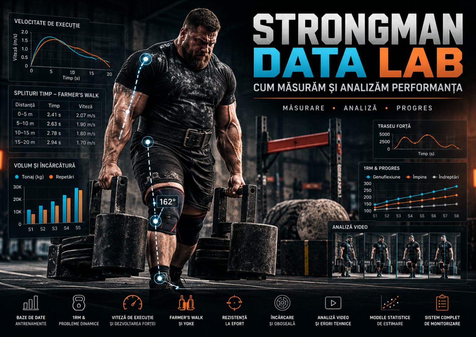
A strongman competition begins long before its opening event. During training, athletes wonder whether they can deadlift a new load, cut two seconds from a Yoke run or turn six Log repetitions into eight. Past results provide clues but never certainty. Outstanding days, injuries, equipment differences and rule changes all complicate the picture. Between what happened and what will happen lies uncertainty, and statistics helps describe it rather than hiding it.

This is Episode Nine of STRONGMAN DATA LAB: HOW WE MEASURE AND ANALYSE PERFORMANCE. After database design, velocity analysis, loaded carries, repeated-event pacing, training-load monitoring and video-based movement analysis, we address a particularly attractive question: can future performance be forecast? We will discuss descriptive statistics, regression, errors, multivariable models, competition predictions and the limitations of artificial intelligence when an athlete has only a small number of comparable results.

We will use explainable models and numerical examples without inventing a universal equation for strongman power. Two Farmer’s courses can have the same length but different surfaces and handles. A conventional Deadlift personal record does not determine the exact outcome using an axle. Predictions only have meaning in relation to event format, rules, time within the season and similarity to the observations underlying the estimate. Strongman biomechanics research documents the diversity of these demands [1], while modern predictive-model reporting emphasises evaluation and transparency [2].

All illustrative athlete cases and numerical datasets constructed in this article are explicitly hypothetical. They do not represent measurements of real identified athletes or experiments conducted by the author. Published references support general methodological principles or particular findings, and transfer from other fields to strongman is identified as an extrapolation. The aim is not to impress with equations but to build a process in which forecasts become testable and prediction error becomes a central finding rather than an embarrassing secret.

1. Prediction is not explanation: two different goals

Explanation seeks to understand mechanisms and relevant relationships. Prediction aims to estimate a future outcome as accurately as possible using information available before that outcome occurs. A model may forecast Farmer’s time from loading, distance and previous performances without proving that any one variable causes changes in speed. Conversely, a sound biomechanical explanation does not necessarily produce an accurate numerical forecast for the next competition.

Suppose Log repetition count correlates with weekly Log training frequency. More experienced competitors may train more frequently while also possessing greater strength, better technique or other advantages. Frequency might be predictive, yet adding two sessions each week would not necessarily cause an equivalent improvement. That would be a causal claim requiring a different research design.

A prediction model can be evaluated by comparing its estimates with outcomes observed later. An explanatory model needs additional consideration of mechanisms, confounding and interventions. The goals can complement one another: theory helps select possible predictors, while forecast errors reveal overlooked factors. Yet they are not synonyms and should not be judged with identical criteria.

For a STRONGMAN DATA LAB, the opening question is what decision the analysis should support. Predicting Yoke time might guide tactics, whereas understanding why Yoke is slow could guide technical training. Without separating these aims, regression coefficients may be turned into unjustified causal coaching instructions.

2. Defining the outcome: what exactly are we forecasting?

A statistical model needs a precisely defined target variable. For Deadlift for Max, the target could be maximum officially accepted load, not the heaviest attempted weight. For Log for Reps, it could be accepted repetition count in seventy-five seconds, not the number of movements started. For Farmer’s, it could be official finishing time under explicit starting and stopping rules. Competition points are another possible target, but those depend on opponents and scoring rules.

An outcome labelled merely «strength» is too broad. An athlete can possess excellent maximal Deadlift strength while struggling with Atlas Stones. A formula based on Squat and Bench does not become a universal predictor of all strongman events. Separate maximal attempts, time-limited repetitions, moving events, loading and medleys. A wider competitive profile can then be constructed without pretending every event expresses the same quality.

Imagine a hypothetical target of official time for a 320 kg Yoke over twenty metres, starting at rest and without additional penalties. Observations at the same mass and distance may be meaningfully comparable if surface and apparatus are similar. A 340 kg run over fifteen metres is a different task unless differences are deliberately modelled. Target definitions should be set before data collection rather than adjusted afterwards to improve results.

Targets can be continuous, such as time or load; discrete counts, such as accepted repetitions; binary, such as success or failure; or ordinal, such as finishing position. Their statistical structures differ. One unchecked linear formula is not automatically appropriate for all, and the choice of method must follow the sporting question.

3. The unit of analysis: repetition, session, athlete or contest?

Within one database, repetitions belong to sets, sets belong to sessions and sessions belong to athletes. Treating every attempt as an independent observation can dramatically exaggerate information content. One hundred repetitions from one athlete are not equivalent to one hundred different athletes. Observations from the same person share anthropometry, training history and many testing conditions.

For predicting an athlete’s future carry time, a standardised run may be the natural unit, while consecutive runs are potentially dependent. For comparing competitors, the unit may be athlete or athlete-in-contest. For predicting individual repetition success, the unit can be the attempt, but its order within a set matters. Each selection changes the interpretation of sample size and uncertainty.

Suppose fifteen athletes each complete twenty Log attempts. The table contains three hundred rows, not three hundred independent people. A random row-level train-test split would place attempts by the same individuals in both subsets. The algorithm might learn individual signatures and appear accurate while failing to generalise to a new competitor. When new-athlete prediction is the purpose, evaluation should separate whole athletes.

For a single-athlete project, time-series dependence becomes important. Sessions close together are not necessarily independent, and programme changes or injuries can affect several consecutive observations. Hierarchical structure is not administrative trivia; it determines whether statistical conclusions are defensible.

4. Data quality comes before algorithms

Sophisticated modelling cannot automatically recover the meaning of inconsistent records. If some Farmer’s entries use kilograms per hand while others use total mass, the algorithm may learn a recording convention rather than a physical relationship. If an invalid Deadlift attempt is entered as a zero-kilogram success, averages become misleading. If one clock begins at the referee’s signal and another at first movement, finishing times may no longer be directly comparable.

A useful register includes athlete identifier, date, event, implement variation, load and unit, distance or duration, official status, timing method and changed conditions. Metadata permit construction of meaningful comparison groups. Before model fitting, check duplicates, impossible values, inconsistent units and missing fields. Missing observations should not all be replaced with zeros.

For example, eleven accepted Log repetitions in sixty seconds and eleven in ninety seconds are different results. The time window must be included before the records can be compared. If event duration is unknown, the record may be unsuitable for a duration-dependent model but should remain in the original archive. Exclusion decisions must be documented rather than made retrospectively to improve a graph.

Transparent reporting of populations and data quality is a principle emphasised in predictive-model guidance [2]. This guidance originates partly in clinical prediction research, not direct validation of strongman models. We apply the general methodological lesson: unclear data provenance produces forecasts that cannot be credibly evaluated.

5. Descriptive statistics: understand distributions before regression

Mean, median, minimum, maximum and dispersion are useful starting points. Consider hypothetical Yoke times of 18.1, 17.8, 18.4, 20.9 and 18.0 seconds. The mean is influenced by the unusually slow run. The median may better describe typical performance, but the unusual attempt should not be hidden. A dropped frame, timing error or genuine control problem would each imply a different interpretation.

Dispersion describes variation as well as average level. Two athletes averaging twenty seconds may differ in consistency: one regularly finishes between 19.8 and 20.2, while another ranges from seventeen to twenty-three. Predictability itself can matter in competition, especially when a very slow run costs placing points. However, variability must be assessed from sufficiently comparable attempts.

Distribution and time-series plots can also reveal data problems. If every performance improves abruptly after an apparatus change, inspect the configuration. If times form two distinct clusters, one may refer to asphalt and another to rubber flooring. Regression across both without accounting for conditions might learn a spurious relationship. Descriptive exploration is a test of whether the modelling question makes sense.

Reports should give observation counts, collection period, conditions and variability. A stand-alone mean can create unwarranted confidence. Sound descriptive statistics provide the foundation for later prediction; they are not disposable introductory material.

6. Measurement error differs from real performance variation

Results vary across days for genuine sporting reasons and because measurement itself is imperfect. Hand timing introduces reaction variation, while video annotation may select different movement-onset frames. The athlete may also alter technique or arrive more fatigued. Atkinson and Nevill described systematic and random error in sports measurements [3]. A model that ignores these components may mistake noise for physiological development.

Imagine Farmer’s time improving from 17.9 to 17.8 seconds. That change might be smaller than timing error. A repeated shift from approximately 18.2 to 16.7 seconds under standardised conditions provides stronger evidence of meaningful performance change. It still does not uniquely identify the adaptation responsible, but measurement uncertainty is less likely to dominate the result.

Reliability should be examined through appropriate repeats, while recognising that consecutive runs can introduce fatigue and familiarisation. Maximal tests are costly; repeated contests should not be organised solely to estimate a standard deviation. Submaximal references and independent timing of identical footage can assess distinct parts of measurement error at lower cost.

Target measurement error constrains the practical ceiling of model performance. If finishing times are measured inconsistently, a complex algorithm may fit quirks of the clocks rather than true capacity. Improving a stable timing protocol can contribute more than adding a neural network.

7. Meaningful change: when should progress alter programming?

Not every numerical difference matters in competition. A tenth of a second at Farmer’s may decide an extremely close placing, but only if timing is reliable enough to resolve that change. One additional Log repetition may change the standings even though count is discrete and can depend on a lockout barely preceding the time limit. Sporting importance and statistical certainty are distinct concepts.

Longitudinal charts may include a band reflecting ordinary test variability, but it should not be called a universal injury threshold or «the limit of progress». When Yoke time appears to improve gradually, assess whether changes exceed typical test fluctuation. If not, monitoring can continue without prematurely declaring success or failure. Lack of clear evidence of improvement is not proof that underlying adaptation is exactly zero.

Sometimes competition rules define practical importance better than a statistical threshold. In Deadlift for Reps, advancing from seven to eight accepted repetitions may matter more than finishing seven a second earlier if only count determines ranking. In other formats, time of last acceptance breaks ties. A useful model predicts outcomes that influence the actual contest.

For each indicator, identify units, known variability and intended decision. This prevents meaningless percentage progress claims. Statistics become useful when connected to real choices, and those choices require both measurement precision and event context.

8. Association between two variables: correlation and its limits

Correlation describes association between variables within a particular sample. For example, athletes with greater Deadlift 1RM may perform better on some repeated-lifting tasks under certain conditions. Yet a between-athlete association is not an individual progression equation. Body mass, experience, rules and participant selection may influence the relationship. Strong correlation does not itself identify a causal mechanism.

Suppose Deadlift 1RM correlates negatively with carry finishing time among ten competitors. That does not prove that increasing one athlete’s Deadlift will proportionally lower their Farmer’s time. Stronger competitors may also be more experienced or technically proficient. Differences in testing conditions could also contribute if equipment was not standardised.

Correlation varies with outliers and the range of values considered. Among elite athletes whose strength levels are similar, an association may appear weaker than in a group spanning beginners to advanced competitors. Neither result is automatically wrong; they describe different populations. Values from one population should not be used for another without assessing compatibility.

A credible report includes sample size, a scatter plot and limitations. Exploratory associations should not be described causally. Correlation may suggest a useful candidate predictor, but the real question is whether it improves forecasts when confronted with new observations.

9. Linear regression: an approximate map between loading and time

Linear regression asks how an outcome changes on average when a measured characteristic changes. With multiple Yoke runs at a fixed distance and different loads, one might model expected time = a + b × load. Coefficient b describes the average change associated with one additional kilogram within the observed range, not a physiological law applying to every athlete. Intercept a may have little practical meaning if zero loading lies far outside the data.

Consider an entirely hypothetical equation: t = 7 + 0.035 × m, where t is time in seconds and m is Yoke mass in kilograms over an unchanged twenty-metre course. The equation predicts 17.5 seconds at 300 kg and 18.2 seconds at 320 kg. These figures follow mathematically from invented coefficients and are not a validated strongman relationship. Coefficients would need to be estimated from real attempts and evaluated on new outcomes before informing competition decisions.

Ordinary linear regression makes assumptions about relationships and errors. When time increases sharply near a competitor’s maximal manageable load, a straight line may underestimate deterioration. Drops and failed finishes complicate matters further. Inspect scatter plots, residuals and coefficient stability. Use a line because it offers a justified approximation in a defined range, not because it makes an attractive chart.

Linear regression’s transparency is a substantial practical advantage. If it consistently fails at heavier loads, acknowledge that domain limitation and investigate alternatives. An understandable model whose weaknesses are visible can be more useful than a complex predictor that nobody can explain when it fails.

10. Residuals: where model limitations become visible

A residual is the difference between observed outcome and model prediction. If a Yoke time of 18.2 seconds is forecast but the athlete finishes in 19.0 seconds, the observed-minus-predicted residual is +0.8 seconds. For time outcomes, a positive residual represents slower-than-predicted performance, while a negative one means faster-than-predicted. It does not mean the athlete was «0.8 seconds more fatigued». The model or measurement could simply be incomplete.

Residual patterns can reveal important omissions. Consistent underestimation above 350 kg suggests a nonlinear load relationship. Larger errors at distances beyond twenty metres suggest including course length. A particular Yoke frame producing unusually large errors suggests apparatus configuration matters. A residual should provoke investigation rather than merely produce a penalty score for the algorithm.

Imagine six observations ordered by increasing load, with errors of −0.2, +0.1, −0.3, +0.2, +1.8 and +2.3 seconds. The two highest-load results suggest the linear model is too optimistic near the upper end. However, six attempts cannot precisely determine the true shape. Document the pattern and gather additional comparable observations before fitting an elaborate curve.

Small residuals on the development dataset do not guarantee future accuracy. The model was fitted precisely to reduce historical errors, so in-sample evaluation is often optimistic. Correctly separated future evaluation data matter far more than celebrating nearly zero error in the same file used for fitting.

11. Multiple regression: value and overfitting risk

Performance depends on more than one variable. Farmer’s time may vary with distance, load per hand, surface, warming-up difficulty and athlete experience. Multiple regression estimates predictive relationships involving several features at once. A simple equation might be time = a + b1 × mass + b2 × distance + b3 × surface category, but coefficients remain dependent on the available data and do not automatically represent causal contributions.

Too many predictors create problems. With eighteen runs and twelve input features, a model may fit coincidences. Predictors may also be correlated: higher loads might be attempted later in the season when the athlete is stronger. Estimated coefficients can become unstable and even change sign when a few attempts are added. The mathematics is not malfunctioning; the data cannot adequately separate effects.

A cautious workflow starts with a small number of sport-relevant variables available before the prediction. For fixed-distance Yoke, load and recent comparable performances might suffice initially. Add a candidate feature only if it improves forecasts on genuinely new attempts. A statistically attractive coefficient from a tiny dataset does not independently justify feature inclusion.

Methods literature on prediction-model sample sizes emphasises dependence on complexity, outcome variation and desired precision [4]. The cited work directly concerns clinical prediction, not strongman, but avoiding overfitting is a transferable statistical principle. There is no defensible universal rule that precisely ten strongman attempts are sufficient for every predictor.

12. Nonlinearity: why ten more kilograms do not always cost the same

At moderate Yoke loading, adding ten kilograms may produce only a small change in finishing time. Near the athlete’s current limit, the same increase may cause stops, altered steps or failure to finish. The true load-time relationship may curve sharply near its upper end. A straight line can miss exactly the region relevant to competition. Its shape cannot be established without enough representative observations.

Polynomial or flexible curves can represent nonlinearity but may behave absurdly outside the measured range. A polynomial may predict negative times or faster results under physically impossible loads. This is a mathematical extrapolation problem, not a discovery about physiology. Constraints can sometimes prevent impossible values, but they must be stated and justified.

For Log for Reps, accepted count may fall steeply as mass increases. If an athlete performs ten repetitions at 90 kg and six at 110 kg, it does not follow that precisely two are available at 130 kg. The relationship is not necessarily linear and may approach a threshold where no repetition is accepted. Models should generally operate within a supported load domain, with strong caution at new extremes.

A highly flexible curve is not always preferable. A table containing several reference points and uncertainty ranges may be more honest and useful. When observed loads occupy a narrow band, data may be unable to distinguish competing plausible functions. Acknowledging that ambiguity protects athletes from decisions based on arbitrary graph shape.

13. Models for repetition count: why counts are special

Accepted repetitions are nonnegative integers. Linear regression might estimate 7.4 repetitions as an expected mean, but an official attempt cannot contain four-tenths of a repetition. An unrestricted linear model might even predict negative counts at extremely heavy loads. Count-model families such as Poisson regression may be considered when their assumptions match the data. Their use should never be automatic.

Timed Log sets have defined windows and a realistic maximum number of cycles. Attempts affect later attempts through fatigue and pacing, so independent events at a constant rate may be an inadequate assumption. A count model might describe mean repetitions while missing their dispersion or the role of failed lifts. An alternative is to model pacing and attempt success separately, if sufficient data are available.

Imagine an athlete repeatedly achieving six, seven or eight accepted Log repetitions at 100 kg over sixty seconds. A model forecasting 7.1 should ideally describe uncertainty and how frequently it expects each integer result. Merely rounding to «seven» conceals meaningful variation. A distribution of possibilities may be more relevant for tactical planning than one number.

With few comparable sets, estimating a complete probability distribution may be unstable. The mean or median of recent trials, accompanied by the observed range, can be a strong benchmark. Advanced modelling becomes worthwhile when it provides demonstrably better forecasts rather than merely a more complicated representation of the same observations.

14. Probability of a valid lift: logistic modelling is not a promise

Some questions are binary: will a particular attempt satisfy the rules? Logistic regression can estimate probability between zero and one using predictors available before the attempt. For heavy Log, candidates might include load, number of completed repetitions, rest duration and previous comparable attempts. But a probability fitted from sparse data is not a direct measurement of the athlete’s physical capacity on competition day.

Suppose a hypothetical model predicts a 0.70 probability of success. This does not mean seventy percent of muscular capacity remains or guarantee seven successes in the next ten attempts irrespective of conditions. It is an estimated frequency implied by a dataset and model. To evaluate it, examine whether attempts assigned roughly seventy-percent success actually succeed at approximately that frequency on independent observations.

A common mistake is including information available only after the target attempt. If the model uses total duration of the lift it is supposed to forecast, impressive statistical performance is possible but useless before the attempt begins. All predictors must genuinely be available at the intended decision time. This basic rule prevents many misleading analyses.

Estimated success probability must never independently authorise dangerous loading. Algorithms can be wrong, and pain, instability or health warning signs cannot be reduced to logistic scores. Prediction may inform tactics only within appropriate technical and safety decisions.

15. Rankings and points: opponents change the target

A strongman may win an event with one performance and finish fifth with an identical result at a stronger contest. Placement is relative rather than an isolated measure of ability. Forecasting event points requires predictions for competitors as well as the specific ranking and tiebreak rules. Points for first place may depend on field size and scoring system.

Imagine a hypothetical contest with eight athletes. Athlete A expects an eighteen-second Yoke finish, while the other seven might finish anywhere between sixteen and twenty-three seconds. A’s placement cannot be determined from their own time alone. If rivals are faster than anticipated, the same result yields fewer points. A model can predict physical time accurately yet perform poorly at predicting ranking.

Five-event competitions are more complex still. A competitor excellent at Deadlift may lose substantial points in Loading Medley. A useful forecast needs event-specific profiles and scoring logic faithful to the actual rules. Published personal records often come from incompatible conditions and should not be treated as interchangeable head-to-head data.

Rank forecasts should be scenarios with uncertainty. Modelling changes in rivals’ performances can reveal how placement sensitivity varies. A possible place in one simulation is not a guaranteed place on the real podium.

16. Baselines: every sophisticated algorithm must beat something simple

Before regression, random forests or neural networks, establish a simple benchmark. For standardised Yoke, it might be the latest valid time or median of the last three comparable runs. For maximal Deadlift, it could be the most recent credible accepted load. For Log for Reps, a typical count from recent matching conditions may suffice. This baseline is the methodological opponent of every more complicated model.

If an application using fifteen features yields mean Yoke error of 1.4 seconds while the three-run median yields 1.0 seconds on the same future trials, the application has not demonstrated better predictive value. It may be technically interesting, but it does not justify adoption for that decision. Methods must be compared on identical evaluation data and under the same error definition, without allowing the complex model privileged knowledge of the future.

Simple baselines can be surprisingly strong for athletes with stable technique and predictable responses. More complex models are useful when genuine multi-variable relationships exist and there are enough observations to learn them. Without those conditions, flexibility becomes the ability to memorise noise. The simple approach is also easy to explain to athletes.

Keep baseline comparisons after every algorithm update. If a new version fails to outperform the reference, do not present it as progress. In applied science, complexity must earn its place through verifiable outcomes.

17. Separating development data from genuine evaluation data

The central question is not how well a model reproduces its history but how accurately it predicts observations it has never seen. Some data must be held outside coefficient fitting and hyperparameter selection. For an individual athlete, future sessions provide the most realistic test. Using October performances to construct a model that supposedly predicted September introduces information from the future into the past.

One illustrative procedure fits the model on the first twenty runs and evaluates the next five, preserving chronological order. That exact split is not universally optimal, but it respects the information available when the prediction would have been made. A rolling-origin approach repeats the process: use observations one through fifteen to predict sixteen, then one through sixteen to predict seventeen, and so forth. This tests forecasts as the athlete’s history grows.

For a model designed for unknown competitors, a different partition is necessary. Entire athletes should be excluded during model development, so their attempts and characteristics do not leak into training. If the same competitors contribute multiple attempts to both training and evaluation subsets, generalisation performance may look unrealistically strong. The model may recognise familiar individuals rather than understanding transferable strongman relationships.

Preprocessing also belongs inside the development process. Feature selection, standardisation, missing-value imputation and threshold tuning should be fitted without inspecting evaluation outcomes. Even calculating one global mean over the entire dataset before splitting can contaminate a supposedly untouched set. Independent evaluation is valuable precisely because its outcomes are a legitimate surprise to the model.

18. Cross-validation helps, but it is not magic

Cross-validation fits and evaluates models over multiple data partitions. It can reduce dependence on one arbitrary split, but it cannot rescue an incorrect definition of independence. Randomly separating repetitions from the same Log set between training and testing gives the model nearly identical context in both subsets. A favourable score may not reflect performance on a future competition day.

The correct scheme follows the intended use. For generalisation to unfamiliar athletes, keep individuals separate across folds. For next-week predictions for one athlete, preserve chronological order. For models intended to forecast results in new competitions, holding entire contests aside may matter because all events within one competition share travel, weather, rules and other contextual factors.

Imagine eighty Farmer’s runs from four competitors. A random run-level split allows the model to learn personal signatures from each athlete. Evaluating the fourth athlete while training only on the first three may produce much larger error. That deterioration is useful evidence. It reveals the distinction between forecasting another attempt by someone already known and forecasting an entirely unfamiliar athlete.

Cross-validation remains an estimate conditional on available data and partition design. It does not turn twenty observations into one hundred independent observations. A dataset from one training season does not guarantee performance two years later after changes in technique, body mass or competition events. Report the exact generalisation question that the method actually tested.

19. Data leakage: when the algorithm secretly sees the future

Data leakage occurs when model development uses information unavailable at the real time of prediction. In sport, it may be subtle. Using the completed session’s RPE to forecast its first attempt supplies information recorded after the target event. A pre-contest ranking forecast cannot include final finishing positions as predictors. The model may look impressive while being impossible to use honestly before the contest.

Leakage also appears during preprocessing. Imagine calculating mean load across development and evaluation data before using that mean to replace missing values in the training set. Information about the supposedly unseen evaluation sample has affected model preparation. The safer workflow learns imputation and scaling rules from development data only and applies them unchanged to new observations.

Duplicate attempts create another route. The same Log clip may appear under two filenames, one entering training and the other evaluation. The algorithm predicts perfectly because it has effectively seen the outcome already. Stable attempt identifiers and duplicate detection are basic requirements of a credible assessment.

Unexpectedly excellent predictive performance should trigger protocol inspection before celebration. Near-perfect results may be possible, but sparse, noisy and heterogeneous strongman data make them especially deserving of scrutiny. The decisive test is future performance on unambiguously independent attempts with reliable measurement.

20. MAE, RMSE and prediction errors athletes can understand

For time prediction, mean absolute error, or MAE, is especially accessible. Take the absolute difference between actual and predicted outcome for each attempt, then average these differences. If four runs have absolute errors of 0.3, 0.7, 1.2 and 0.6 seconds, MAE is 0.7 seconds. It shares the outcome’s unit and is straightforward to communicate.

Root mean squared error, RMSE, gives greater weight to large misses. A contest strategy model that occasionally misses a Yoke time by five seconds may be problematic even when most estimates are good. MAE and RMSE offer complementary perspectives, and reports should not confuse them, particularly when comparing samples with different distributions.

For repetition counts, MAE is measured in repetitions. For maximal lift predictions, it is expressed in kilograms. For binary successful-attempt predictions, probability-focused metrics are needed, not merely percent classifications correct. A score may classify most attempts correctly by always predicting success in a dataset dominated by successful submaximal lifts, while providing poor information about difficult attempts.

Always report evaluation error, number of predictions, loading range and baseline performance. If a model misses Yoke times by 1.5 seconds on average but standings are separated by 0.2 seconds, its tactical value may be limited. Predictive error should be judged in the units and decisions that matter to the athlete.

21. Why R-squared is not enough

R² is popular because it summarises how much outcome variation a model captures within a particular sample relative to a statistical reference. Yet a high training-set R² does not guarantee reliable forecasts. A flexible curve can pass extremely close to historical points and fail on the next attempt. In-sample fit must therefore be accompanied by independent or time-ordered evaluation.

R² also depends strongly on the outcome range. In a dataset containing Yoke times from ten to sixty seconds, a model may account for much of the broad variation while still missing individual runs by several seconds. Among elite competitors completing runs between seventeen and nineteen seconds, the same absolute error might produce a much worse R². That does not automatically make the second model less useful for a concrete competition decision.

Out-of-sample R² can even be negative when model predictions are worse than the appropriate simple reference. Such results should not be hidden or replaced with zero to improve presentation. They show that the model has limitations or does not generalise to the evaluated population. MAE, RMSE, individual errors and systematic bias should be inspected alongside R².

We should avoid claims such as «the model explains ninety-five percent of the athlete’s strength» when R² comes from a handful of training sessions. Outcome, loading domain and evaluation sample all require explanation. A statistic can be mathematically correct and still be interpreted badly in sporting language.

22. Prediction intervals: future outcomes are not single numbers

A point forecast may say that an athlete will finish a Yoke course in 18.5 seconds. Comparable future performances can vary because of readiness, technique, apparatus and other factors. A prediction interval attempts to describe a range that may contain a future observation under stated assumptions and coverage goals. This differs from a confidence interval for the estimated mean, which concerns uncertainty about an average rather than an individual future result.

An entirely hypothetical model might estimate 18.5 seconds with an illustrative prediction interval of 16.9 to 20.4 seconds. The figures are not empirical findings. They show why making tactical choices solely from the midpoint may be fragile. Even a reasonable model can be followed by an unusually slow run, and contest conditions may move the result beyond the interval.

Meaningful intervals require enough representative observations and a method suited to the error distribution. A claimed ninety-percent interval derived from only five attempts may have unreliable actual coverage. Theoretical coverage must be tested on new data rather than equated automatically with the frequency achieved in strongman settings.

Wide intervals are sometimes the correct answer. They reveal that the available data cannot support the desired precision. Narrowing them artificially to make the forecast attractive defeats their purpose. Explicit uncertainty can be more useful than an exact-looking number because it shows which decisions remain reasonable across a range of plausible outcomes.

23. Probability calibration: what makes a success model credible?

A probability model might assign an eighty-percent chance that an athlete completes another valid repetition. Calibration asks whether attempts receiving similar probabilities succeed at roughly the advertised frequency. If attempts predicted near eighty percent succeed only half the time on new data, the model is too optimistic. A model can rank successful attempts above failures while still providing poorly calibrated probabilities.

This matters for competition tactics. When deciding whether to attempt another lift in the final ten seconds, an inflated probability may exaggerate expected benefit. Yet probability should never replace safety assessment. Pain, instability or clinical warning signs are not cancelled by a display reading «92% likelihood of success».

Imagine ten future attempts assigned a predicted success probability of 0.70, with seven accepted. This is compatible with calibration near seventy percent but far too small for strong confidence. Six successes would not automatically prove a defect either, because random variation is substantial. Calibration requires adequate data volume and explicit uncertainty.

Clubs with very few comparable attempts may be better served by cautious descriptive categories than precise percentages, provided the categories are defined and useful. «Insufficient data to estimate reliably» is often more responsible than «73.8% probability». The model must support decisions without manufacturing certainty.

24. Performance time series: progress is rarely a straight line

An athlete may improve rapidly during the opening of a block, stagnate halfway through and produce excellent results after recovery. A straight trend line through all sessions can hide this structure and forecast competition day poorly. Time series need interpretation alongside training phases, workloads and context. Regressing performance on calendar date does not prove each day adds a fixed quantity of strength.

Imagine Farmer’s times gradually improving over eight weeks but worsening during weeks four and five because of a high-volume block. A date-only model may treat those changes as noise without representing the planned training structure. Adding training phase might improve forecasts, but that must be demonstrated rather than assumed. The predictor also has to be known before the outcome.

Some changes are intentional. Off-season hypertrophy work may not aim for weekly Yoke records. A deload may temporarily improve bar speed through lower acute fatigue. Models ignoring block purpose can misinterpret intermediate results as failure and suggest unsuitable changes.

A practical time-series approach might use a moving median or short-window trend. But choosing the window after inspecting which one fits best can itself create overfitting. Time-ordered evaluation of successive forecasts is needed before claiming predictive improvement. Individual development is a sequence of adaptation and context, not an obligation to follow an elegant statistical line.

25. Moving averages and continuously updated forecasts

Moving averages are among the most accessible tools for athletes who collect consistent data. Instead of relying equally on attempts from the last three years, calculate the mean or median of the latest three to five comparable trials. The aim is to describe recent ability and update the estimate as training progresses. Window choice creates a trade-off: short windows respond quickly but amplify noise, while longer windows are steadier but slow to recognise genuine change.

Consider hypothetical twenty-metre Farmer’s times at 110 kg per hand: 18.2, 17.8, 18.0, 17.4, 17.6 and 17.2 seconds. The last three average 17.4 seconds, whereas all six average about 17.7. These numbers answer slightly different questions. The first represents recent results, the second includes more distant history. Neither is a guarantee about the next attempt.

Moving statistics should be presented alongside variability and labels for changes of apparatus or programme. If three fast runs used a new course, they should not simply replace older observations without checking conditions. If one session occurred just after competition, retain the context rather than silently discarding it solely to obtain a favourable trend.

For many practical coaching decisions, this simple approach may be sufficient. When a complex predictor does not outperform the recent-trial median on future attempts, there is little reason to add administrative burden. Monitoring should reduce decision-relevant uncertainty rather than maximise mathematical complexity for its own sake.

26. Learning from small datasets: regularisation offers limited protection

When numerous features compete for few observations, model coefficients can become unstable. Regularisation penalises complexity or large coefficient values and can reduce some forms of overfitting. Ridge and LASSO are well-known approaches; Tibshirani’s original LASSO work described coefficient shrinkage and selection [5]. Such techniques do not create new evidence. They introduce constraints in an attempt to improve generalisation.

A Farmer’s model might use mass, distance, body mass, RPE, pickup time and recent training history. With only ten runs, estimating several separate effects can become highly sensitive to one data point. Regularisation may stabilise predictions but cannot establish that selected features are causal determinants of performance. Coefficients also depend on the chosen penalty and observed population.

The amount of regularisation should be selected through a valid development procedure, without repeatedly consulting untouched future outcomes. If dozens of versions are tested and the one performing best at a completed contest is selected retrospectively, the selection process has itself been overfitted. Final evaluation must remain separate from optimisation.

For one athlete with many standardised sessions, regularisation may be useful. With five comparable Log attempts, it cannot turn an inadequate dataset into a reliable repetition forecast. Reducing predictors and gathering more relevant observations may be better than switching algorithms.

27. Random forests: flexibility without sporting magic

Random forests combine many decision trees for prediction or classification. Breiman’s foundational paper [6] formalised an approach capable of representing nonlinear relationships and interactions without requiring one linear equation. For strongman, the method could explore links among Yoke loading, distance, experience and conditions. Flexibility still requires enough representative data and proper evaluation on unseen outcomes.

A tree may learn rules such as «when load exceeds 340 kg and distance exceeds twenty metres, expected finishing time increases». Such thresholds may reflect peculiarities of the sample rather than genuine performance boundaries. With little data, a tree may memorise attempts and an ensemble may only partly reduce this instability. Each split is not a biomechanical law or coaching prescription.

Feature-importance rankings require equal caution. If body mass appears important, it does not follow that changing an individual athlete’s weight will produce the forecasted result. Body mass may be associated with strength, experience or competitive category. Prediction and intervention are different questions, and algorithmic complexity does not remove causal confounding.

Before adoption, compare a forest with simple regression and a baseline on future trials. If extra predictive value is small or absent, the transparency of a simpler model can be preferable. Machine learning should earn its place through demonstrated usefulness rather than a more fashionable name than «median of the last three runs».

28. Neural networks and the limits of small strongman datasets

Neural networks can represent flexible relationships and process complex inputs, including video sequences and time-series signals. With large, consistently labelled image datasets, such systems may be promising. But a gym holding twenty Yoke runs and ten Log sets does not possess sufficient evidence to justify training a large bespoke numerical forecasting model from scratch. Memorisation and failure on new attempts are serious risks.

Pretrained pose-estimation systems introduce another issue: their outputs must be checked under large implements, unusual postures and changing camera views. Episode Eight showed how an incorrectly inferred anatomical landmark can produce precise-looking but invalid angle estimates. Feeding those numbers into a second model propagates the original uncertainty rather than cancelling it. Sophisticated forecasting can still depend on weak measurements.

Explainability matters for decisions. If a network recommends reducing Log loading by ten kilograms, the coach needs to understand the evidence, intended outcome and uncertainty behind that recommendation. An impressive score without independent evaluation cannot replace technical judgment or the athlete’s condition. Automating a fragile conclusion does not make it safer.

For most club-level strongman projects, simple well-tested algorithms may currently be the better option. If future databases contain thousands of comparable attempts and independent evaluation sets, the trade-off can be reassessed. Technology should follow a question it can answer, not arrive before there are data adequate to support an answer.

29. Grouped observations and athlete-specific effects

In multi-athlete datasets, results from the same individual are generally more related than results from different people. Hierarchical or mixed-effects models can represent both common relationships and individual differences when data support them. A Yoke model might allow each athlete a separate baseline finishing time while estimating an overall association with loading. This is more realistic than assuming every competitor has the same starting performance.

Such a model can describe an average loading relationship and variation around it for individual athletes. With only three competitors and a few runs, however, individual-effect estimates will be highly uncertain. A hierarchical formula is not a substitute for an adequate sample. Statistical structure organises the information that exists; it does not invent additional participants.

Suppose one athlete improves Farmer’s performance while another remains stable. A group average may show modest progress and conceal these differing trajectories. Individual-effect modelling can make them visible, but causal conclusions still depend on programmes, loads and other context. A statistical date effect does not prove every session within the period was effective.

The prediction objective also determines evaluation. Forecasting another attempt for a known athlete differs from forecasting a completely new athlete. Models may perform very differently in these scenarios. Time-ordered testing suits known-athlete forecasting, whereas group separation is essential for claims of generalisation to unfamiliar competitors.

30. Transfer between events: what does Deadlift predict about Atlas?

Strongman combines events with partially overlapping demands. Hip extension, trunk control, grip and technical skill may influence multiple events in different proportions. A large Deadlift 1RM may matter for some object lifts without determining Atlas Stones or Farmer’s outcomes. Cross-event relationships require empirical examination. Strongman biomechanics research [1] documents that these movements are not interchangeable versions of one task.

To investigate transfer, examine results from the same athletes across documented events and conditions. A correlation between Deadlift and Sandbag Pickup may suggest shared physical requirements, but does not prove that improving one will necessarily improve the other. Body size, technique and experience may explain some of the relationship. Associations between athletes should not be automatically applied to progression within one individual.

Imagine a hypothetical athlete increasing Deadlift from 250 to 270 kg while loading a 120 kg Atlas Stone in nearly unchanged time. This does not make the strength gain worthless. Atlas performance may be constrained by object positioning or transition to extension. A Deadlift-only predictor misses the event’s specific demands and therefore makes an inaccurate forecast.

A robust system can retain separate profiles for maximal pulling, loaded travel, overhead pressing and object loading. Cross-event features can be added only when sufficient data show improved future prediction. Theoretical appeal is not enough. Transfer is a hypothesis to examine, not a guaranteed consequence of higher numbers in related exercises.

31. Competition data and participant selection bias

Published contest results appear attractive for statistical models because outcomes are official and competitively relevant. Yet participants are selected: athletes must be invited or register, reach the venue, remain healthy enough to compete and satisfy the rules. Analysing only finishers excludes withdrawals and unsuccessful efforts, potentially creating an incomplete picture. This is a representativeness problem, not merely a shortage of observations.

Competitors also make strategic load choices. Someone may decline a further maximal attempt because enough points have been secured; another may attempt an unrealistic load to recover places. The highest accepted weight is a genuine competition outcome but not always the precise physiological maximum. Modelling it as a perfect measure of capacity ignores tactics.

A model built mainly from elite competitors may be unsuitable for beginners. A dataset dominated by very heavy athletes may not generalise to lightweight categories. Age, experience, apparatus and rules influence the population to which a forecast applies. Model reporting should describe participants rather than only average results.

For a new contest, examine whether the athletes and event formats resemble those underlying the model. When equipment information is incomplete or the event is unusual, uncertainty should be communicated explicitly. A precise-looking forecast cannot repair missing representativeness.

32. Missing observations, withdrawals and DNF results

Strongman competitors may fail to finish a carry within the time limit or receive no accepted repetition. These outcomes should not be treated as ordinary zero-second finishing times. If someone covers only twelve of twenty metres before the sixty-second limit, the complete finishing time was not observed. Record completed distance, time limit and DNF status instead of inventing the unobserved outcome.

Excluding every non-finish can make a time model overly optimistic by retaining only successful attempts. Replacing every DNF with exactly sixty seconds assumes that all would have finished then, which may be false. Methods for censored outcomes or separate modelling of finish probability may be more appropriate when sufficient data exist. The chosen method should match how the competition actually scores non-finishes.

Missing video is not the same as DNF. A broken camera does not mean the athlete failed the event. Status fields can distinguish nonparticipation, nonfinish, official invalidation, absent measurement and medically prompted withdrawal. These distinctions prevent absurd conclusions, including treating an unmeasured run of zero seconds as a new record.

With sparse data, robust statistical solutions may be unavailable for every missingness pattern. Limit the scope of the model where necessary and disclose how many observations were excluded and why. Transparency is better than filling gaps with imaginary performances no one observed.

33. Hypothetical case study: predicting Deadlift for Max

Consider an athlete preparing for maximal Deadlift with recent submaximal sets and two accepted maxima. A hypothetical training log contains three repetitions at 240 kg with RPE 8, two at 250 kg with RPE 9 and a previously accepted 270 kg single. These observations do not automatically guarantee that 280 kg will be available in competition. Relationships among repetitions, perceived effort and maximal strength vary across athletes and exercise variants.

A simple model might use the latest accepted maximum as its baseline and treat recent sets as contextual information. If it estimates a competition result of 275 kg, the calculation and its limitations must be explained. A broad illustrative range, perhaps 260 to 285 kg, could express uncertainty, but should not be presented as a statistically calibrated prediction interval without evaluating errors across adequate comparable contests.

Attempt selection is a separate tactical question. The opener may seek a secure valid result, the second attempt a competitive placing and the third an improvement conditional on opponents. Even a perfect prediction of final capacity would not automatically determine optimal sequencing without success probabilities, scoring rules and competition context. Estimating capacity is not the same as providing a complete attempt strategy.

If the athlete eventually validates 265 kg, record the forecasting error and any known reason for failed attempts. Do not retrospectively change the original forecast to 265 and claim success. Retaining estimates issued before competition creates an auditable record and permits genuine comparison against the last-accepted-result baseline.

The analysis should also note whether competition equipment matched training. An axle, elevated starting position or different approved equipment can alter the task. A prediction for conventional Deadlift is not independently validated for every strongman variant merely because the load is expressed in kilograms.

34. Hypothetical case study: Farmer’s mean and tactical uncertainty

A competitor prepares for a twenty-metre Farmer’s event at 130 kg per hand. Five comparable hypothetical runs take 17.2, 17.9, 16.8, 18.1 and 17.4 seconds. Their mean is about 17.5 seconds, while observed times span 1.3 seconds. A forecast of 17.5 is a reasonable reference but does not guarantee the next run will be close to average. Competition tactics may depend on how much variability the athlete accepts through an aggressive start.

Suppose video reveals drops during the slower runs. A model including the actual number of drops may explain historic times extremely well, but it cannot use future drop count as a predictor before the next race. Instead, prior drop frequency, loading and starting conditions may be available. The distinction between advance information and an intermediate outcome occurring later is essential.

A more elaborate model could estimate both the chance of finishing without a drop and expected time if no drop occurs. That requires enough observations in both categories. If the athlete has only one dropped run across twenty attempts, detailed probability estimates may be highly unstable. A modest point forecast plus a clearly labelled dropped-implement scenario may be more useful.

After competition, compare official time, stops and deviation from the estimate. If the prediction failed because the surface differed, preserve the context. One slow race does not prove the athlete regressed. A model can fail on one day and still have long-term utility, but that claim must be supported by accumulated out-of-sample errors.

It is also worth recording whether the performance target concerns speed alone or successful completion under control. Some strategies increase average speed while increasing the chance of a drop. A useful model should not treat the fastest isolated result as the only outcome of interest when inconsistency changes likely competition points.

35. Hypothetical case study: Log for Reps and final-attempt probability

Imagine a 110 kg Log event lasting seventy-five seconds. Recent comparable training sets yielded six, seven, six and seven accepted repetitions, with variable inter-repetition intervals. A simple reference would forecast six or seven. A more complex model might use times of the first three lockouts and perceived effort, but those variables are available only after the event starts. Pre-event prediction and live in-event updating are distinct tasks.

Suppose the third repetition is accepted at second thirty-one. A model might update its estimate for reaching seven repetitions, but any probability requires adequate comparable training data. Four previous sets cannot justify a precise figure such as «78.6%». A more defensible response is to describe the observed range and discuss tactics consistent with the athlete’s known behaviour.

Early pace may predict final count while also reflecting strategy. One athlete may begin slowly to preserve capacity for later efforts, while another loses an opportunity to complete an additional lift. Treating the first three repetition timestamps as simple causes of final count would ignore differences in loading and pacing intention. Tactical models need evaluation under specific rules on genuinely new sets.

During competition, complex real-time graphics may distract from implement control and judging commands. The main value of statistical work may be before the event: practising a reliable pace, reviewing failed attempts and understanding typical variability. Data support tactics without replacing physical control or referee decisions.

The final analysis should preserve both accepted and rejected attempts. A forecast that predicts count correctly but repeatedly misses the mechanism of time loss may have limited coaching value. Predictive accuracy and technical explanation are complementary questions, not the same achievement.

36. Hypothetical case study: extrapolating heavy Yoke from lighter loads

An athlete records twenty-metre Yoke times of 15.2 seconds at 260 kg, 16.8 at 300 kg and 19.1 at 340 kg. A simple fitted line may suggest a result at 360 kg. But the final increment could produce stops or instability that fundamentally changes the relationship. Three observations do not justify a complex nonlinear curve. The 360 kg prediction must be labelled extrapolation, not near-certain performance.

Suppose the simple estimate is 20.3 seconds, while the athlete completes the course in 23.0. The miss does not prove the entire idea of modelling is worthless. Perhaps loading crossed a threshold where the athlete’s usual technique became difficult to maintain. Equipment, readiness or course conditions may also have changed. Examine context and whether similar errors recur at heavy loads.

A responsible report might state conditional scenarios: if pacing remains comparable to previous runs, time may be near the estimate; if stops occur, the forecast becomes unreliable. Do not convert those statements into calibrated probability intervals unless the data support that procedure. Sometimes the most useful statistical conclusion is that there are too few observations near competition loading.

Additional testing still carries a fatigue cost. Repeated maximal Yoke runs should not be prescribed merely to improve model coefficients. An intermediate submaximal reference or a technical run already planned can reduce uncertainty at a more reasonable cost. Decision quality should be balanced against the physical cost of collecting new evidence.

37. Competition simulation: multiple event forecasts become a ranking

For a five-event strongman contest, a basic simulator can take estimated outcomes for every competitor, apply official rankings and calculate total points. Probabilistic simulation additionally needs outcome variability rather than only expected values. The goal is to explore scenarios in which an athlete rises or falls in placing, not to claim that the future has been mathematically fixed.

A wholly hypothetical field of eight athletes across five events could generate thousands of possible finishing-time and lifting-result combinations if plausible distributions were available for everyone. Each simulated contest produces scores under the stated rules, and repeated simulations yield a distribution of rankings. But a large number of simulations does not make the initial assumptions correct. One can simulate a false premise a million times and merely obtain a very repeatable mistake.

Dependence between events matters. Injury, unusual fatigue or tactical conservation can affect several consecutive results. A simulator assuming complete independence may understate such scenarios. Rule-specific event order can also influence outcomes. Assumptions about correlations and tactical choices should be stated and tested against historical competitions where possible.

For a small club, three transparent scenarios may be more honest than precise invented probabilities: favourable, central and difficult. These can reveal where points might be gained and which events have substantial uncertainty. The analysis can inform preparation without masquerading as a validated podium-probability model.

A simulator should also handle ties and DNFs faithfully. Ranking algorithms that award the wrong number of points under shared placings can materially distort final standings even when performance predictions are accurate. Scoring logic requires the same care as the statistical model.

38. Monte Carlo: a million simulations cannot repair weak inputs

Monte Carlo simulation repeatedly draws hypothetical values from specified distributions and calculates the resulting outcomes. The method is useful for exploring uncertainty, but its answers depend on the assumptions supplied. Incorrect Farmer’s variability or exclusion of possible non-finishes may produce overly optimistic rankings. More simulation iterations reduce computational sampling error, not the error caused by a poor input model.

In an illustrative scenario, an athlete’s Yoke time is modelled around nineteen seconds with some run-to-run variability. Many plausible times can be generated and compared with estimated opponents. But if rivals’ records come from different surfaces or course lengths, the selected distributions may not represent the real contest. The precision of the podium percentage depends chiefly on competitor data, not processing power.

Sensitivity analysis provides an important safeguard. If changing one assumption slightly moves estimated podium probability from fifteen to sixty percent, the forecast is fragile. A single figure such as «42.3%» should not be reported without describing that dependence. It may be more informative to state that ranking uncertainty is dominated by incomplete knowledge of opponents.

A reproducible simulation states its data sources, ranking rules, handling of ties, DNFs and event dependence. When these elements are unavailable, explicitly labelled teaching scenarios are appropriate. Numbers generated from convenient assumptions are not observed results of a validated model.

Even when all inputs are documented, simulation is not a replacement for official competition information. Event loads, starting order and rules can change. Model scenarios should be updated when confirmed details become available, while old forecasts are retained for genuine evaluation.

39. Season-long evaluation: the frozen-forecast diary

An effective way to avoid convenient hindsight is to preserve forecasts before each contest. Record date, time, model version, available information, expected outcome and any uncertainty range. After the event, add official result and calculate prediction error. Do not alter the original estimate to make it resemble reality. This discipline creates an auditable history of model performance.

Suppose there are ten pre-event forecasts for Deadlift for Reps. The model overpredicts twice and underpredicts three times. Examine the distribution of errors, not just their average signed value. Positive and negative mistakes can cancel, producing a near-zero mean despite poor accuracy in individual contests. Absolute and signed errors should therefore be reported separately.

Forecasts for events the athlete ultimately does not attempt should also be preserved with an accurate status. Medical withdrawal or logistical absence is not a zero-kilogram result or a zero-second finish. Separate unevaluable forecasts from prediction errors on events that actually occurred. Otherwise, outcome selection can distort reported accuracy.

At season end, compare the new method with the simple baseline on the same contests. Modest but repeated improvements may justify continued use. Instability may favour simplification. A system that acknowledges its misses is more valuable than one publishing only successful forecasts.

Archive how predictions were communicated to the athlete as well. If an estimate was originally described as highly uncertain, it should not later be judged as though it was a confident guarantee. Consistent documentation protects both scientific interpretation and honest coaching communication.

40. Detecting regime changes: when history stops representing the athlete

Athletes change technique, experience injuries, gain or lose body mass and move between training phases. In those situations, distant history may become less representative of current capability. Time-series methods can sometimes identify changes in level or variability, but cannot automatically assign a cause. Context is necessary to decide whether the predictive model needs recalibration.

Imagine a Log technique change followed by shorter clean times across six consecutive sessions. A model based mostly on older attempts might underpredict current performance. A documented change date or stronger weighting of recent observations might help, but these choices need prospective evaluation. Old results should not simply be erased to create a more attractive trend.

Conversely, one outstanding result after a recovery week does not prove a permanent capacity increase. An excessively reactive model may update forecasts too aggressively and suggest unsuitable loads. There is a balance between adaptation to change and forecast stability, and the choice depends on how costly particular errors are for the athlete.

Major changes in implement, rules, technique and training phase should therefore be logged. When future outcomes systematically depart from predictions, investigate whether the underlying process changed before adding arbitrary features. Sometimes the model is not intrinsically «bad»; it was built for an athlete whose present conditions no longer resemble the original collection period.

41. Prediction and training-load monitoring: a tempting but fragile connection

With session RPE, tonnage and fixed-reference performance data, coaches may try to forecast how an athlete will perform after different training weeks. The attractive goal is knowing when volume will support adaptation and when its fatigue cost becomes excessive. Yet relationships among loading, fatigue and adaptation are complex. Two weeks with identical internal-load totals may contain very different exercises and distributions [7]. No simple formula guarantees accurate prediction of the physiological response.

Imagine slower Yoke times after weeks above 3,500 AU and faster results following weeks below 2,500 AU. A simple association might suggest that higher load «harms» performance. However, the athlete may be in a planned accumulation block, with adaptation expressed after recovery. A model ignoring programme timing might recommend less training precisely when productive stimulus is needed.

Lagged models can explore relationships between one week’s exposure and later performance. Selecting the lag from sparse historical data may create chance associations, and retrospective fit does not establish prospective usefulness. Evaluate forecasts on future weeks under rules chosen in advance. Changes of programme and important symptoms also require independent consideration, regardless of predictions.

No workload-derived score should be treated as a medical diagnosis of overtraining or an exact injury-risk probability. Load-management consensus documents emphasise context and multiple sources of evidence [8], while critiques of acute-to-chronic ratios describe substantial conceptual and statistical weaknesses [9]. Performance modelling may support training decisions, but health and safety require separate appropriate assessment.

42. Decisions under uncertainty: when strategies look equally plausible

One model may suggest an aggressive Farmer’s start saves 0.3 seconds on average but increases variability and stopping risk. Another may favour a more conservative start with slightly slower expected time but greater consistency. The best choice depends on what the competition rewards: absolute time, reliable completion or points relative to rivals. A predictor does not define the tactical objective by itself.

Imagine a hypothetical contest in which an athlete needs first place in Yoke to reach the podium. A more aggressive but technically controlled strategy might have value if second or third does not improve overall ranking. In another situation, merely finishing validly may preserve the current position, making consistency more attractive. Both discussions must remain within technical control and safety constraints.

Possible results can be translated into points under explicit rules, exploring outcomes of each strategy. If a conservative approach often secures a decent placement while an aggressive approach sometimes wins but sometimes fails, the trade-off becomes visible. Without adequate data, do not attach precise probabilities to these scenarios. It is possible to reason about consequences without pretending to know their likelihood exactly.

A sound decision process begins by identifying the goal and unacceptable outcomes, including preventable loss of control and ignored injury warnings. Prediction then helps compare the remaining options. Statistical analysis does not remove responsibility for final decisions; it makes the trade-offs more explicit and open to scrutiny.

43. A four-week protocol for a first prediction model

In week one, select one narrow question, such as finishing time for a twenty-metre Farmer’s course at a standardised load. Fix the rules, timing procedure, apparatus and required fields. Review historical attempts and document exclusions for incompatible conditions. Choose a simple baseline, perhaps the median of the most recent three comparable runs. Avoid rushing into an elaborate multi-model experiment.

In week two, inspect the outcome distribution and fit a simple model if there are enough observations. Examine whether previous finishing time predicts the next attempt or whether variations in load add useful information. Define in advance how error will be measured on future attempts. With only four comparable records, recognise that rigorous evaluation is not yet possible and keep collecting appropriate observations.

During week three, record a forecast before a run already included in the athlete’s training plan. Preserve its timestamp, version and estimate. Compare it with the actual result afterwards without rewriting history. If the error is large, first check whether surface, handles or session fatigue differed. One run cannot establish model success or failure, and maximal testing should not be added solely to populate the dataset.

In week four, compare accumulated forecasting errors with those of the simple baseline. Simplify if the new model does not improve performance. If results appear consistently better, maintain the procedure and gather more evidence before making public validity claims. Four weeks are a methodological exercise, not proof of universal accuracy. The goal is learning a reliable forecasting discipline.

The same process can later be extended to Deadlift or Log, but each new target requires its own operational definitions. Do not assume that a model successful for a fixed Farmer’s course will transfer directly to maximal lifting. Starting narrowly makes data quality and error interpretation easier to manage.

44. What a research-quality prediction report contains

A credible report identifies the population, collection period, events, target definition, available predictors, apparatus and excluded results. It then describes model fitting, data partitioning, error metrics and comparison against a simple reference. Probability models require calibration assessment; continuous forecasts need examination of individual errors and justified uncertainty intervals. Readers should understand how the development data differ from the intended deployment setting.

TRIPOD+AI provides detailed reporting guidance for predictive models developed using regression or machine learning in clinical research [2]. It is not a strongman-specific validation standard, but its principles of transparency transfer well. Reporting only an algorithm’s most favourable score without numbers of observations or evaluation procedure is insufficient. Credibility requires describing both methods and limitations.

A responsible illustrative statement might read: «In a hypothetical dataset of forty comparable runs, model A achieved MAE of 0.9 seconds on the final eight, compared with 1.1 seconds for the three-run median». Even that difference requires caution due to small evaluation size and changing conditions. It should not be turned into a dramatic percentage claim without explaining precisely what was compared.

Include an observation-level error table when appropriate while protecting unnecessary personal information. Real athlete data require suitable permissions, while constructed examples need explicit labelling. Models with substantial error may still be scientifically informative by revealing missing features or weaknesses in measurement procedures.

A report should also explain intended use and non-use. A model that estimates a future time is not a medical clearance tool or a replacement for the coach’s judgement. A forecast developed for moderate training loads should not be advertised as reliable for unfamiliar competition maxima. These boundary statements are part of reproducibility.

45. Prediction as coaching communication, not a verdict

An athlete seeing «Yoke 19.5 seconds» may interpret the number as a promise. The coach should explain that it is conditional on specified circumstances and that changes in loading or surface may alter the outcome. Present a credible uncertainty interval where available. If no calibrated interval exists, state that the estimate is only a descriptive reference rather than dressing it up as certainty.

When the forecast is less ambitious than the athlete’s goal, do not reduce their aspirations to the algorithm’s number. Explain that the current historical record does not support a more optimistic forecast, while subsequent training can change the evidence available. A harder goal may still be tested appropriately in the programme with consideration for technique and safety. The model offers partial evidence, not authority over athletic ambition.

When the forecast is exceptionally favourable, loading should not rise automatically. The result may reflect a run of good days, while recovery and training-phase objectives remain important. Statistical predictions should not encourage unplanned maximal attempts, especially when control issues or symptoms arise. Their value lies in realistic expectations and identification of information gaps.

An effective conversation combines expected result, uncertainty and a next action: «record two more comparable runs», «examine the pickup», or «repeat the reference after recovery». The model becomes a shared learning instrument. It is an estimate the athlete and coach can confirm, reject or refine rather than a permanent judgement displayed by software.

Coaches should remain careful with language when the forecast is wrong. Calling the athlete a disappointment because a prediction was missed confuses model uncertainty with personal failure. The appropriate response is to review the measurement and assumptions, and then adjust the method if repeated evidence warrants it.

46. Limits of strongman-specific predictive research

Strongman does not yet offer the same breadth of standardised datasets found in some sports with highly uniform competition formats. Apparatus, distances, loading, surfaces and rules change frequently. Two competitions both labelled «Yoke Walk» are not necessarily comparable. The 2019 biomechanical review describes limited direct literature for many events [1]. We should not claim that one universal predictive equation has been validated across the entire discipline.

Future research could prospectively record standardised loading, distances, times, invalid attempts, technical indicators and competition outcomes. It should include athletes across relevant experience levels, with participant characteristics accurately described. Evaluation needs genuinely independent contests or athletes. Otherwise, sophisticated models risk being little more than elegant summaries of their own development data.

Studies could also examine whether technology genuinely adds predictive value. Does video-derived timing improve forecasts beyond a simple stopwatch? Does recent perceived exertion improve next-session prediction? Do hierarchical models outperform the most recent accepted result when forecasting a new athlete? These questions should be specified before evaluation, and negative findings reported as transparently as positive ones.

Until stronger evidence exists, incremental development is appropriate: define the task, collect reliably, test a simple baseline and evaluate repeatedly on future performances. A modest, auditable model is more scientific than naming a score calculated from a few incompatible trials «artificial intelligence for sports performance».

Research can also benefit from data dictionaries and shared event taxonomies across clubs, subject to consent and privacy. Common definitions of valid attempts, time limits and implement configurations would make comparisons more meaningful. Standardisation does not mean ignoring event diversity; it means describing that diversity consistently enough for analysis.

47. Ethics of prediction: athlete labels and apparent certainty

Models estimating competition winners can inform tactical exploration, but may also create unfair labels when deployed without context. Athletes with fewer contests or limited access to equipment have less data and greater predictive uncertainty. Labelling them as «without potential» because their dataset is sparse confuses missing information with lack of ability. Forecasts should be conditional estimates, not judgements about human worth.

When models compare weight classes, experience levels or sexes, examine whether prediction error differs across relevant groups. A favourable overall average can hide systematic error among underrepresented athletes. If the sample is too small to evaluate subgroup performance, disclose the limitation rather than assuming fairness. Transparency is both a statistical and an ethical requirement.

Personal data, videos and health information require protection. A sporting model should not automatically incorporate sensitive medical records or publish private training history without appropriate rights and consent. Aggregate methodological results can often be described without revealing identifiable participants. The scientific value of a predictor does not depend on making every private data point public.

Communication should avoid definitive conclusions about talent, intelligence or character based on results. Athletes can improve through training, technical learning, recovery and experience, while models can be updated as new evidence arrives. The statistical virtue is being able to revise hypotheses rather than convert a probability estimate into a permanent identity.

Athletes should also understand how estimates are used. A coach may reasonably use a forecast to discuss pacing, but automatic selection exclusion or public ranking based on untested predictions raises a different level of concern. The more consequential the decision, the stronger the required evidence and human review should be.

48. Conclusion: forecast carefully, never manufacture certainty

Performance estimation is possible within limits, but it does not mean predicting future results with guaranteed precision. Models learn from observations influenced by rules, technique, implements, training and measurement error. Linear regression can be useful, random forests can represent interactions, and simulations can explore possible rankings. None is more reliable than the data and independent evaluation supporting it.

Strongman specificity is fundamental: there is no single coefficient converting Deadlift into Atlas, Log into Viking Press or Yoke into Farmer’s. Official results, testing conditions and individual variation must be preserved. Forecasts become meaningful when evaluated against future attempts and compared with simple baselines. A documented forecasting error is more valuable than a perfect score produced by leakage from the evaluation data.

In a mature STRONGMAN DATA LAB, forecasts are issued before attempts with explicit limits, then compared against observed results. The difference is recorded, plausible explanations are investigated and methods are revised only after appropriate checks. A coach who knows when the model is uncertain may make better decisions than one impressed by an exact-looking decimal. Stating uncertainty makes science useful rather than weak.

Episode Ten will conclude the series by integrating all the components into a complete strongman decision system: indicators, dashboard structure, data collection, validation, forecasting and training-programme review. From a filmed repetition to the planning of an entire season, the objective remains unchanged: measure carefully, interpret in proportion to evidence and keep the athlete rather than the algorithm at the centre of performance.

Scientific bibliography

[1] Hindle, B. R., Lorimer, A., Winwood, P., & Keogh, J. W. L. (2019). The Biomechanics and Applications of Strongman Exercises: A Systematic Review. Sports Medicine - Open, 5, 49. https://doi.org/10.1186/s40798-019-0222-z

[2] Collins, G. S., Moons, K. G. M., Dhiman, P., et al. (2024). TRIPOD+AI Statement: Updated Guidance for Reporting Clinical Prediction Models That Use Regression or Machine Learning Methods. BMJ, 385, e078378. https://doi.org/10.1136/bmj-2023-078378

[3] Atkinson, G., & Nevill, A. M. (1998). Statistical Methods for Assessing Measurement Error (Reliability) in Variables Relevant to Sports Medicine. Sports Medicine, 26(4), 217–238. https://doi.org/10.2165/00007256-199826040-00002

[4] Riley, R. D., Ensor, J., Snell, K. I. E., et al. (2020). Calculating the Sample Size Required for Developing a Clinical Prediction Model. BMJ, 368, m441. https://doi.org/10.1136/bmj.m441

[5] Tibshirani, R. (1996). Regression Shrinkage and Selection via the Lasso. Journal of the Royal Statistical Society: Series B (Methodological), 58(1), 267–288. https://doi.org/10.1111/j.2517-6161.1996.tb02080.x

[6] Breiman, L. (2001). Random Forests. Machine Learning, 45, 5–32. https://doi.org/10.1023/A:1010933404324

[7] Bourdon, P. C., Cardinale, M., Murray, A., et al. (2017). Monitoring Athlete Training Loads: Consensus Statement. International Journal of Sports Physiology and Performance, 12(Suppl 2), S2-161–S2-170. https://doi.org/10.1123/IJSPP.2017-0208

[8] Soligard, T., Schwellnus, M., Alonso, J. M., et al. (2016). How Much Is Too Much? (Part 1) International Olympic Committee Consensus Statement on Load in Sport and Risk of Injury. British Journal of Sports Medicine, 50(17), 1030–1041. https://doi.org/10.1136/bjsports-2016-096581

[9] Impellizzeri, F. M., Tenan, M. S., Kempton, T., Novak, A., & Coutts, A. J. (2020). Acute:Chronic Workload Ratio: Conceptual Issues and Fundamental Pitfalls. International Journal of Sports Physiology and Performance, 15(6), 907–913. https://doi.org/10.1123/ijspp.2019-0864

[10] Bland, J. M., & Altman, D. G. (1986). Statistical Methods for Assessing Agreement Between Two Methods of Clinical Measurement. The Lancet, 327(8476), 307–310. https://doi.org/10.1016/S0140-6736(86)90837-8

[11] Sánchez-Medina, L., & González-Badillo, J. J. (2011). Velocity Loss as an Indicator of Neuromuscular Fatigue During Resistance Training. Medicine & Science in Sports & Exercise, 43(9), 1725–1734. https://doi.org/10.1249/MSS.0b013e318213f880

[12] Pareja-Blanco, F., Rodríguez-Rosell, D., Sánchez-Medina, L., et al. (2017). Effects of Velocity Loss During Resistance Training on Athletic Performance, Strength Gains and Muscle Adaptations. Scandinavian Journal of Medicine & Science in Sports, 27(7), 724–735. https://doi.org/10.1111/sms.12678